Home < Documentation < Nightly < Modules < HeterogeneityCAD
Introduction and Acknowledgements
|
Extension: OpenCAD
This work is supported by NA-MIC, NCIGT, and the Slicer Community.
Author: Vivek Narayan, Jayender Jagadeesan
Contact: Jayender Jagadeesan <email> jayender@bwh.harvard.edu</email>
|
|
This project is supported by P41 RR019703/RR/NCRR NIH HHS/United States, P01 CA067165/CA/NCI NIH HHS/United States and P41 EB015898/EB/NIBIB NIH HHS/United States
|
Module Description
The HeterogeneityCAD module is an image feature extraction toolbox primarily to quantify the heterogeneity of tumor images and their label maps. Source code for batch processing without the GUI is also included at the end of this document.
Navigating the Module
- HeterogeneityCAD Input
- Add Volume Node to the Nodes List
- Nodes can be either grayscale volumes or parameter maps (Volumes or Label Maps)
- Individual Nodes can be added be selecting a volume in the Drop-down menu and clicking 'Add Node'
- 'Add All Nodes from Scene' adds all volumes and labels in the scene
- Individual Nodes in the Nodes List can be removed by selecting them and clicking 'Remove Node'
- All Nodes in the Nodes List can be removed by clicking 'Remove All Nodes'
- A corresponding Label Map must also be selected to use as as the Region Of Interest (ROI)
|
|
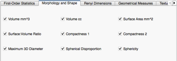
- HeterogeneityCAD Metrics Selection
- Each tab menu corresponds to a list of metrics for a feature class (First-Order Statistics, Morphology and Shape, Renyi Dimensions...)
- An individual metric can be included or excluded from the computation by checking or unchecking its checkbox
- For some feature classes, unchecking the critical computations (in bold) will disable the other metrics
- Right-Clicking on a metric will open a description and a menu for editing metric parameters
- i.e. in the adjacent Figure right-clicking on the 'Mean Intensity' metric displays a description and a parameter menu
|
|
- HeterogeneityCAD Metrics Output and Summary
- Clicking 'Apply HeterogeneityCAD' begins computation of the selected metrics for every Node in the Nodes List
- A Progress Bar will show the Node and which feature class of metrics is currently being computed
- Calculations for Renyi Dimensions, Geometrical Measures, and Texture metrics may take a longer time to compute depending on the size of the ROI
- After the computations, a table will be displayed
- i.e. in Figure 3, each row will represent a Node, and each column will display the output of each selected metric
- Clicking 'Save to File' will prompt the user to save the table information as a Comma-Separated value (CSV) File
|
|
Data sets
Quick Instructions for Use
- Add an image or parameter map (.nrrd file) to the Nodes List
- Select a corresponding segmentation label map to use as ROI
- Click "Apply HeterogeneityCAD"
Image Features and Metrics
- First-Order and Distribution Statistics
- Data Node: The name of the input node - either an image volume or parameter map.
- Voxel Count: The total number of voxels within the ROI of the grayscale image or parameter map.
- Energy: A measure of the magnitude of values in an image. A greater amount larger values implies a greater sum of the squares of these values.
- Entropy: Specifies the uncertainty in the image values. It measures the average amount of information required to encode the image values
- Minimum Intensity: The value of the voxel(s) in the image ROI with the least value.
- Maximum Intensity: The value of the voxel(s) in the image ROI with the greatest value.
- Mean Intensity: The mean of the intensity or parameter values within the image ROI.
- Median Intensity: The median of the intensity or parameter values within the image ROI.
- Range: The difference between the highest and lowest voxel values within the image ROI.
- Mean Deviation: The mean of the distances of each image value from the mean of all the values in the image ROI.
- Root Mean Square: The square-root of the mean of the squares of the values in the image ROI. It is another measure of the magnitude of the image values.
- Standard Deviation: Measures the amount of variation or dispersion from the mean of the values in the image ROI.
- Skewness: Measures the asymmetry of the distribution of values in the image ROI about the mean of the values. Depending on where the tail is elongated and the mass of the distribution is concentrated, this value can be positive or negative.
- Kurtosis: A measure of the 'peakedness' of the distribution of values in the image ROI. A higher kurtosis implies that the mass of the distribution is concentrated towards the tail(s) rather than towards the mean. A lower kurtosis implies the reverse, that the mass of the distribution is concentrated towards a spike the mean.
- Variance: The mean of the squared distances of each value in the image ROI from the mean of the values. This is a measure of the spread of the distribution about the mean.
- Uniformity: A measure of the sum of the squares of each discrete value in the image ROI. This is a measure of the heterogeneity of an image, where a greater uniformity implies a greater heterogeneity or a greater range of discrete image values.
|
|
- Shape and Morphology Metrics
- Volume mm^3: The volume of the specified ROI of the image in cubic millimeters.
- Volume cc: The volume of the specified ROI of the image in cubic centimeters.
- Surface Area mm^2: The surface area of the specified ROI of the image in square millimeters.
- Surface:Volume Ratio: The ratio of the surface area (square millimeters) to the volume (cubic millimeters) of the specified ROI of the image.
- Compactness 1: A dimensionless measure, independent of scale and orientation. Compactness 1 is defined as the ratio of volume to the (surface area)^(1.5). This is a measure of the compactness of the shape of the image ROI
- Compactness 2: a dimensionless measure, independent of scale and orientation. This is a measure of the compactness of the shape of the image ROI.
- Maximum 3D Diameter: The maximum, pairwise euclidean distance between surface voxels of the image ROI.
- Spherical Disproportion: The ratio of the surface area of the image ROI to the surface area of a sphere with the same volume as the image ROI.
- Sphericity: A measure of the roundness or spherical nature of the image ROI, where the sphericity of a sphere is the maximum value of 1.
|
 Shape and Morphology Metrics |
- Renyi Dimensions
- Box-Counting Dimension: Part of the family of Renyi Dimensions, where q=0 for Renyi Entropy calculations. This represents the fractal dimension or the slope of the curve on a plot of log(N) vs. log(1/s) where 'N' is the number of boxes occupied by the image ROI at each scale, 's', of an overlaid grid.
- Information Dimension: Part of the family of Renyi Dimensions, where q=1 for Renyi Entropy calculations.
- Correlation Dimension: Part of the family of Renyi Dimensions, where q=2 for Renyi Entropy calculations.
|
|
- Geometrical Measures
- Extruded Surface Area: The surface area of the binary object when the image ROI is "extruded" into 4D, where the parameter or intensity value defines the shape of the Fourth dimension.
- Extruded Volume: The volume of the binary object when the image ROI is 'extruded' into 4D, where the parameter or intensity value defines the shape of the Fourth dimension
- Extruded Surface:Volume Ratio: The ratio of the surface area to the volume of the binary object when the image ROI is 'extruded' into 4D, where the parameter or intensity value defines the shape of the Fourth dimension.
- Extruded Box-Dimension:
|
|
- Texture: Gray-Level Co-occurrence Matrix (GLCM)
- Autocorrelation: A measure of the magnitude of the fineness and coarseness of texture.
- Cluster Prominence: A measure of the skewness and asymmetry of the GLCM. A higher values implies more asymmetry about the mean value while a lower value indicates a peak around the mean value and less variation about the mean.
- Cluster Shade: A measure of the skewness and uniformity of the GLCM. A higher cluster shade implies greater asymmetry.
- Cluster Tendency: Indicates the number of potential clusters present in the image.
- Contrast: A measure of the local intensity variation, favoring P(i,j) values away from the diagonal (i != j), with a larger value correlating with larger image variation.
- Correlation: A value between 0 (uncorrelated) and 1 (perfectly correlated) showing the linear dependency of gray level values in the GLCM. For a symmetrical GLCM, ux = uy (means of px and py) and sigx = sigy (standard deviations of px and py).
- Difference Entropy:
- Dissimilarity:
- Energy (GLCM): Also known as the Angular Second Moment and is a measure of the homogeneity of an image. A homogeneous image will contain less discrete gray levels, producing a GLCM with fewer but relatively greater values of P(i,j), and a greater sum of the squares.
- Entropy(GLCM): Indicates the uncertainty of the GLCM. It measures the average amount of information required to encode the image values.
- Homogeneity 1: A measure of local homogeneity that increases with less contrast in the window.
- Homogeneity 2: A measure of local homogeneity.
- Informational Measure of Correlation 1 (IMC1):
- Informational Measure of Correlation 2 (IMC2):
- Inverse Difference Moment Normalized (IDMN): A measure of the local homogeneity of an image. IDMN weights are the inverse of the Contrast weights (decreasing exponentially from the diagonal i=j in the GLCM). Unlike Homogeneity 2, IDMN normalizes the square of the difference between values by dividing over the square of the total number of discrete values.
- Inverse Difference Normalized (IDN): Another measure of the local homogeneity of an image. Unlike Homogeneity 1, IDN normalizes the difference between the values by dividing over the total number of discrete values.
- Inverse Variance:
- Maximum Probability:
- Sum Average:
- Sum Entropy:
- Sum Variance: Weights elements that differ from the average value of the GLCM.
- Variance (GLCM): The dispersion of the parameter values around the mean of the combinations of reference and neighborhood pixels, with values farther from the mean weighted higher. A high variance indicates greater distances of values from the mean.
|
|
- Texture: Gray-Level Run Length Matrix (GLRL)
- Short Run Emphasis (SRE): A measure of the distribution of short run lengths, with a greater value indicative of shorter run lengths and more fine textural textures.
- Long Run Emphasis (LRE): A measure of the distribution of long run lengths, with a greater value indicative of longer run lengths and more coarse structural textures.
- Gray Level Non-Uniformity (GLN): Measures the similarity of gray-level intensity values in the image, where a lower GLN value correlates with a greater similarity in intensity values.
- Run Length Non-Uniformity (RLN): Measures the similarity of run lengths throughout the image, with a lower value indicating more homogeneity among run lengths in the image.
- Run Percentage (RP): Measures the homogeneity and distribution of runs of an image for a certain direction
- Low Gray Level Run Emphasis (LGLRE): Measures the distribution of low gray-level values, with a higher value indicating a greater concentration of low gray-level values in the image.
- High Gray Level Run Emphasis (HGLRE): Measures the distribution of the higher gray-level values, with a higher value indicating a greater concentration of high gray-level values in the image.
- Short Run Low Gray Level Emphasis (SRLGLE): Measures the joint distribution of shorter run lengths with lower gray-level values.
- Short Run High Gray Level Emphasis (SRHGLE): Measures the joint distribution of shorter run lengths with higher gray-level values.
- Long Run Low Gray Level Emphasis (LRLGLE): Measures the joint distribution of long run lengths with lower gray-level values.
- Long Run High Gray Level Emphasis (LRHGLE)Measures the joint distribution of long run lengths with higher gray-level values.
|
|
Similar Modules
Label Statistics
References
- J. Jayender, E. Gombos, S. Chikarmane, D. Dabydeen, F. A. Jolesz, and K. G. Vosburgh, “Statistical Learning Algorithm for In-situ and Invasive Breast Carcinoma Segmentation”, Journal of Computerized Medical Imaging and Graphics, vol. 37, no. 4, pp. 281-292, 2013
- J. Jayender, S. A. Chikarmane, F. A. Jolesz and E. Gombos, “Automatic Segmentation of Invasive Breast Carcinomas from DCE-MRI using Time Series Analysis”, Journal of MRI, Article first published online 23 September 2013, doi: 10.1002/jmri.24394
- J. Jayender, K.G. Vosburgh, E. Gombos, A. Ashraf, D. Kontos, S.C. Gavenonis, F. A. Jolesz and K. Pohl , “Automatic Segmentation of Breast Carcinomas from DCE-MRI using a Statistical Learning Algorithm”, IEEE International Symposium on Biomedical Imaging, pp. 122-125, 2012.
- J. Jayender, D.T. Ruan, V. Narayan, N. Agrawal, F. A. Jolesz and H. Mamata, “Segmentation of Parathyroid Tumors from DCE-MRI using Linear Dynamic System Analysis”, IEEE International Symposium on Biomedical Imaging, 2013.
- J. Jayender, J. Jagannathan, S.Chikarmane, C.P.Raut and F.A. Jolesz, “Computer-Aided Diagnosis of Breast Angiosarcoma: Results in 14 cases”, Quantitative Medical Imaging Symposium, 2013 (invited paper).
- HJWL Aerts, ER Velazquez, RTH Leijenaar, et al., "Decoding tumour phenotype by noninvasive imaging using a quantitative radiomics approach", vol. 5, Nat Communication, 2014.
Information for Developers
To be added so that developers can add their metrics. Also, we are validating the metrics - please use caution while using them.
Download from: https://github.com/vnarayan13/Slicer-OpenCAD
Source code: https://github.com/vnarayan13/Slicer-OpenCAD/tree/master/HeterogeneityCAD
Source code for batch processing: https://github.com/Slicer-OpenCAD/HeterogeneityCADScript
[Use the TestScript.bash script for batch processing]


