Difference between revisions of "Modules:FourDAnalysis-Documentation-3.5"
| Line 150: | Line 150: | ||
Customize following [http://viewvc.slicer.org/viewcvs.cgi/ links] for your module. | Customize following [http://viewvc.slicer.org/viewcvs.cgi/ links] for your module. | ||
| − | [http://www.na-mic.org/Slicer/Documentation/Slicer3/html/ Links] to documentation generated by doxygen. | + | [http://www.na-mic.org/Slicer/Documentation/Slicer3-doc/html/ Links] to documentation generated by doxygen. |
== More Information == | == More Information == | ||
Latest revision as of 23:05, 15 January 2010
Home < Modules:FourDAnalysis-Documentation-3.5Return to Slicer 3.5 Documentation
Module Name
4D Analysis Module
General Information
Module Type & Category
Type: Interactive
Category: 4D
Authors, Collaborators & Contact
- Junichi Tokuda, Ph.D., Brigham and Women's Hospital
- Wendy J Plesniak, Ph.D., Brigham and Women's Hospital
- Ron Kikinis, M.D., Brigham and Women's Hospital
- Hiroto Hatabu, M.D., Ph.D., Brigham and Women's Hospital
Contact: Junichi Tokuda, tokuda at bwh.harvard.edu
Module Description
The 4D Analysis Module allows you to analyze a time-series of 3D images (4D image) on 3D Slicer. Currently, the module offers the following features:
- Intensity plot. The module can draw intensity curves at the specified regions of interest.
- Pharmacokinetic model analysis. (SciPy required) The users can perform pharmacokinetic model analysis based on the intensity curves. Models are defined in Python scripts so that the users can modify the existing models or create their own pharmacokinetic models.
- Parameter map. (SciPy required) The module also allows generating a map of pharmacokinetic parameters.
In default, only the intensity plot is available. To use the other functions, you need to install scipy for 3D Slicer and recompile 4D Analysis module. Please refer the section bellow for more detail.
Usage
Quick Tour of Features and Use
Basic features
- Active 4D Bundle: Specify the active 4D image.
- Frame Control: View the 4D image data. 4D images can be loaded from 4D Image Module.
- Intensity Plot: Generate intensity curves and display them on this panel. The curves are measured for each labeled region in the specified label map. If the label map contains multiple labels, the module generates intensity curve for each label. The user can also load/save curves from/to CSV files. The plotting graph can be controlled from Python interactor or other 3D Slicer modules. See Slicer3:2DPlotting for more detail.
Advanced features (require SciPy installation)
- Model/Parameter: Select Python script and parameters for pharmacokinetic analysis.
- Curve Fitting: Perform a single curve fitting. It displays the result parameters.
- Parameter Map: Generate parameter map. The module performs curve fitting for each voxel in the specified region.
Tutorial 1: Plotting time-intensity curve from 4D image data
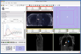
The module allows plotting mean intensities in the specified region on the series of images.
Step 1: Load 4D image
Please follow 4D Image module documentation page to load time-series image data.
Step 2: Define a mask
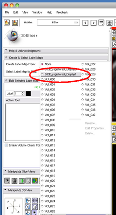
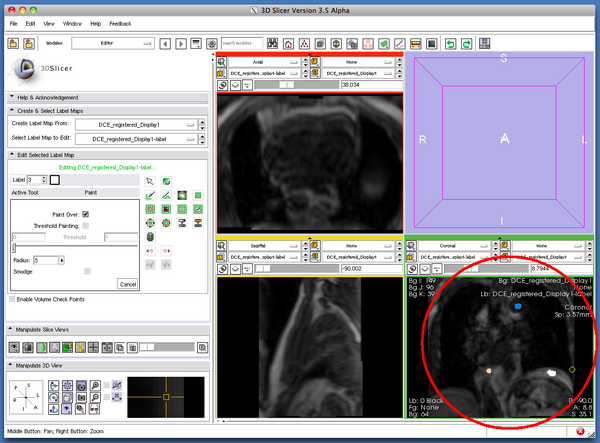
After loading 4D image from 4D Image module, open Editor and make a label map to mask regions you want to measure mean intensities. When you make a label map, please specify one of display volume nodes created by 4D Image module (a volume node with a name "*_Display1") (Figure 2-3).
Step 3: Plot
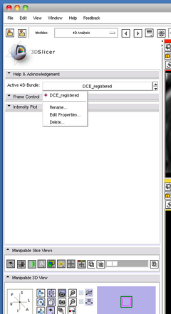
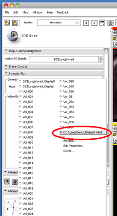
Open 4D Analysis module in 4D category, and choose the 4D image loaded in the first step from Active 4D Bundle node selector menu (Figure 4). If you have only one 4D image loaded on your Slicer, it should be already there.
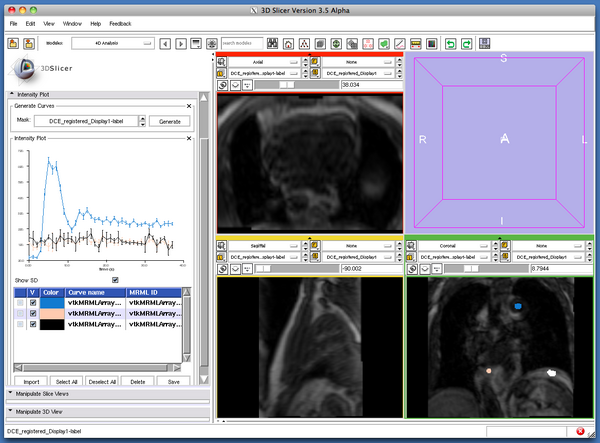
After specifying the 4D image, open Intensity Plot tab and select the mask volume, which you created in the previous step (Figure 5), and then press Generate' button. If you have multiple labels in the label volume, the module generates time-intensity curves for each label (Figure 6).
Step 4: Show and hide curves
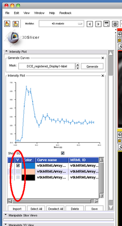
The column list bellow the graph allows you to show and hide the curves by clicking the check boxes in the V column.
Step 5: Save intensity curve data
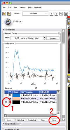
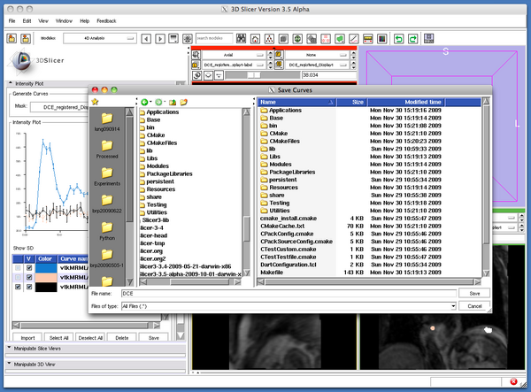
To save the plot data as CSV files, turn on the check boxes in the left column of the curves to save in the column list, and then click the Save button bellow the column list (Figure 8). The Slicer will pop up a dialog window (Figure 9). The curve data is stored in CSV files, which can be loaded to 4D Analysis Module later.
Step 6: Delete intensity curve data
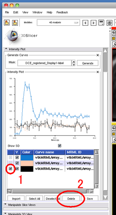
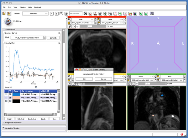
To delete the plot data, turn on the check boxes in the left column of the curves to delete in the column list, and then click the Delete button bellow the column list (Figure 10). The Slicer will pop up a confirmation dialog box(Figure 11).
Development
Setting up SciPy-based curve analysis
The module offers several intensity curve analysis methods. Currently those methods are implemented based on Python SciPy package, which does not come with 3D Slicer in default. If you are interested in trying them, please follow the steps bellow:
Step 1: Install SciPy
Please refer Slicer3 Python page. We have a good experience to build SciPy with 3D Slicer in Mac OS X 10.5; you just install GNU Fortran complier, turn on USE_SCIPY option in slicer_variables.tcl in the source directory and then run Scripts/getbuildtest.tcl to build 3D Slicer. You can get Fortran binary at R for Mac OS X Developer's Page. You may try the same on Linux, but the build script may not work well in some Linux environment.
Step 2: Building 4D Analysis module with SciPy Option
If you haven't built 3D Slicer yet, edit Line 11 in FourDAnalysis/CMakeLists.txt as follows:
007:
008: # --------------------------------------------------------------------------
009: # Option: use Scipy for curve fitting (SciPy must be installed)
010:
011: option(FourDAnalysis_USE_SCIPY "Use SciPy for curve fitting." ON)
012:
then run getbuildtest.tcl script.
If you have already built 3D Slicer, you can set FourDAnalysis_USE_SCIPY "ON" by running make with edit_cache option:
$ cd <Slicer3-build directory>
$ cd Modules/FourDAnalysis
$ make edit_cache
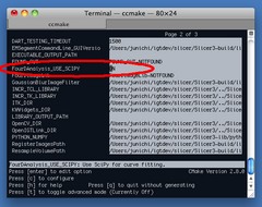
Make program will launch ccmake (full screen CMake configuration tool) (Figure 12), where you can turn on FourDAnalysis_USE_SCIPY macro. After generating a new make file, quit ccmake screen and run make.
After building the module, run 3D Slicer to check if the 4D Analysis module has been built with SciPy option.
Dependencies
The intensity curve analysis functions depend on SciPy package. Please turn on SciPy option when you build your 3D Slicer.
Known bugs
Follow this link to the Slicer3 bug tracker.
Usability issues
Follow this link to the Slicer3 bug tracker. Please select the usability issue category when browsing or contributing.
Source code & documentation
Customize following links for your module.
Links to documentation generated by doxygen.
More Information
2D Graph
The module provides a set of classes to support 2D Graph for intensity curve plotting, which can potentially be used for other projects. Please refer Slicer3:2DPlotting for more detail.
Acknowledgment
This work is supported by NIH (5R21CA116271: Dynamic contrast-enhanced MRI of pulmonary nodule at 3T, PI: Hiroto Hatabu), NA-MIC, and NCIGT.
