Documentation/Nightly/Modules/ShapeVariationAnalyzer
|
For the latest Slicer documentation, visit the read-the-docs. |
Introduction and Acknowledgements
|
Extension: ShapeVariationAnalyzer Authors: Mateo Lopez (university of North Carolina) and Priscille de Dumast (University of Michigan) License: Apache License, Version 2.0 |
|

Module Description
Shape Variation Analyzer (SVA) allows the computation of PCA decomposition of groups of shapes in order be able to represent them in a lower dimensional space. SVA also allows the user to explore the generated PCA space and to evaluate the quality of the generated models. The aim of this extension is to help understand morphological variations.
The module is composed of multiple panels to perform the different steps of the process: create the groups, pre-visualize the groups and update them if necessary, generate explore and evaluate the generated models.
Use Cases


Tutorials
Requirements
- Windows
To use this extension on Windows, you must run 3D Slicer as administrator.
- MacOS
Mac OS 10.11.0 or later
- Linux
Prerequisities
Both the 3D models into the training dataset and those to classify must have the same number of points. The most correspondent the shapes are, the better it is for the computation. This can be performed thanks to ShapeAnalysisModule and improved with RigidAlignment/Groups.
Creation of CSV File

|
This tab allows the user to create a CSV file gathering all the VTK file paths and their corresponding group. |
 |
 |
 |
|
Add Group
Add one by one the directories containing the VTK files for each group. |
Modify Group
Each group can be edited, with a modification of its corresponding repository. |
Remove Group
Only the last group added can be removed. |
Preview/Update of the classification groups

|
This tab allows the visualization of the 3D models in ShapePopulationViewer, and update the group assigned to the shapes if needed. |
- Preview with ShapePopulationViewer

|
|
Generating and saving the models
This step will compute the PCA model of each group and will save those models for a future exploration.You’ll need to provide the CSV file which contains the groups.
- Perform the computation
- Load the CSV file containing the groups if you haven't performed the previous steps
- Clic on Process and Export
- The exploration interface will appear, it gives you all the tools to explore the generated models.
- Save the models
- Clic on save exploration.
- Choose the folder in wich the exploration should be saved and give it a name (ex: 'exploration-name.json').
- Saving the exploration will create files as follow:
Average shapes : exploration-name_[i]_mean.vtk
PYC file : exploration-name.pyc
- Load an exploration
To load an exploration select a JSON file previously generated ('exploration-name.json') in the JSON File field.
Model Exploration

This section is divided into 3 part:
- The PCA exploration
- The color modes description and parameterization
- The plots visualization and interaction
The PCA exploration
To start exploring a PCA space, select the group you want to explore in the group option.
Use the sliders to see the shape transform. Each slider represent an eigenvalue of the PCA model, the explained variance value represent how significant this eigenvalue is compared to the other ones.
If you want to play with more sliders, you can use the 'Minimum Explained Variance' and 'Maximum Number of eigenvalues' parameters:
- The 'Minimum Explained Variance' parameter will make appear only sliders that have a higher explained variance than the defined value.
- The 'Maximum Number of eigenvalues' parameter is the maximum number of sliders that can be displayed.
If you want to see (or hide) the mean shape of the group in a superposition of the current shape, you can use the 'toggle mean shape' option.
The color modes description and parameterization


There are 3 different color modes to visualize the current shape that can be selected in the Color Mode parameter:
- the group color mode
- the unsigned distance to mean shape mode
- the signed distance to mean shape mode
- The group color mode:
This mode will display the shape with the color associated with his group.
To change the color of a group, click on the white colored square next to the group selection and select a new color.
- The unsigned distance to mean shape mode
This mode will display, at each point of the shape, a color representing the unsigned distance between the point and the corresponding point of the group mean shape.
The color scale used is white(0) to red(maximal distance). You can change the color range (ie: the maximal distance) by using the Maximum distance parameter.
- The signed distance to mean shape mode
This mode will display, at each point of the shape, a color representing the signed distance between the point and the corresponding point of the group mean shape.
The color scale used is blue(minimal distance) to white(0) to red(maximal distance). You can change the color range (ie: the maximal or minimal distance) by using the Maximum distance and Minimal distance parameter. In any case, the white color is fixed to a 0 distance.
A distance will be signed negatively if the associated point is inside the mean shape of the group and positively if the associated point is outside the mean shape of the group.
The plots visualization and interaction
After generation of the models, 2 plots are available:- The Variance plot
- The Projection plot (interactive)
If an evaluation of the models has been processed, 3 other plots are available:

- The Generalization plot
- The Specification plot
- The Compactness plot
We describe them in the Model Evaluation section.
They can be visualized by selecting the corresponding plot chart in the plot area menu (top left button of the plot area).


- The Variance plot
This plot shows, for the selected group, the explained variance ratio of each eigenvalue in a bar plot and the cumulated sum of the explained variance ratio in a scatter plot.
The number of components displayed corresponds to the number of sliders available.
- The Projection plot (interactive)
This plot shows the projection on the 2 first component of the selected group.
You can interact with this plot using a point selection mode ('select points' or 'freehand select points') available in the interaction mode option of the plot area menu.
Selecting one point on this plot will modify the sliders values to show the corresponding shape in the 3D window.
If you select more than 1 point, the mean shape of all the selected points will be displayed.
The point selection modifies ALL the sliders, even those who are not displayed on the interface. if you want to show the shape only using the displayed sliders and not the other ones, you can uncheck the 'Use hidden eigenmodes' option, at the bottom of the sliders.
Model Evaluation
To evaluate the generated models, 3 values can be computed:- The generalization
- The specificity
- The compactness
two parameters are available for the evaluation. one is the number of random shapes that have to be generated to compute the specificity. The other one is defined by the number of sliders currently available if we have 8 sliders, the evaluation is computed on 8 components.
To launch the evaluation, use the Evaluate models option. As the evaluation of the models can take a long time, you have the possibility to abort the evaluation by using the same button.
Visualize the evaluation
When the evaluation is completed, 3 new plots are available in the plot area, one for each value.
You can visualize them by choosing the corresponding plot chart in the plot area menu.
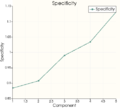
Specificity
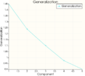
Generalization
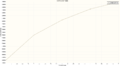
Compactness


Similar Modules
N/A
References
N/A
Information for Developers
The source code of this module is available on GitHub: https://github.com/DCBIA-OrthoLab/ShapeVariationAnalyzer