Home < Modules:MRIBiasFieldCorrection-Documentation-3.6Return to Slicer 3.6 Documentation
Gallery of New Features
Module Name
MRIBiasFieldCorrection
General Information
Module Type & Category
Type: CLI
Category: Filtering
Authors, Collaborators & Contact
- Sylvain Jaume: MIT CSAIL
- Nicolas Rannou: ISEN IRISA
- Ron Kikinis: Harvard Medical School SPL
- Contact: sylvain at csail.mit.edu
|
|
- Step 1/24. Select input image:
- Input Image: input image
- Mask Image: label map providing an approximative segmentation of the ROI
- Output Volume: corrected image
|
|
- Step 2/24. Select mask image:
- Input Image: input image
- Mask Image: label map providing an approximative segmentation of the ROI
- Output Volume: corrected image
|
|
- Step 3/24. :
- Input Image: input image
- Mask Image: label map providing an approximative segmentation of the ROI
- Output Volume: corrected image
|
|
- Step 4/24. :
- Input Image: input image
- Mask Image: label map providing an approximative segmentation of the ROI
- Output Volume: corrected image
|
|
- Step 5/24. :
- Input Image: input image
- Mask Image: label map providing an approximative segmentation of the ROI
- Output Volume: corrected image
|
|
- Step 6/24. :
- Input Image: input image
- Mask Image: label map providing an approximative segmentation of the ROI
- Output Volume: corrected image
|
|
- Step 7/24. :
- Input Image: input image
- Mask Image: label map providing an approximative segmentation of the ROI
- Output Volume: corrected image
|
|
- Step 8/24. :
- Input Image: input image
- Mask Image: label map providing an approximative segmentation of the ROI
- Output Volume: corrected image
|
|
- Step 9/24. :
- Input Image: input image
- Mask Image: label map providing an approximative segmentation of the ROI
- Output Volume: corrected image
|
|
- Step 10/24. :
- Input Image: input image
- Mask Image: label map providing an approximative segmentation of the ROI
- Output Volume: corrected image
|
|
- Step 11/24. :
- Input Image: input image
- Mask Image: label map providing an approximative segmentation of the ROI
- Output Volume: corrected image
|
|
- Step 12/24. :
- Input Image: input image
- Mask Image: label map providing an approximative segmentation of the ROI
- Output Volume: corrected image
|
|
- Step 13/24. :
- Input Image: input image
- Mask Image: label map providing an approximative segmentation of the ROI
- Output Volume: corrected image
|
|
- Step 14/24. :
- Input Image: input image
- Mask Image: label map providing an approximative segmentation of the ROI
- Output Volume: corrected image
|
|
- Step 15/24. :
- Input Image: input image
- Mask Image: label map providing an approximative segmentation of the ROI
- Output Volume: corrected image
|
|
- Step 16/24. :
- Input Image: input image
- Mask Image: label map providing an approximative segmentation of the ROI
- Output Volume: corrected image
|
|
- Step 17/24. :
- Input Image: input image
- Mask Image: label map providing an approximative segmentation of the ROI
- Output Volume: corrected image
|
|
- Step 18/24. :
- Input Image: input image
- Mask Image: label map providing an approximative segmentation of the ROI
- Output Volume: corrected image
|
|
- Step 19/24. :
- Input Image: input image
- Mask Image: label map providing an approximative segmentation of the ROI
- Output Volume: corrected image
|
|
- Step 20/24. :
- Input Image: input image
- Mask Image: label map providing an approximative segmentation of the ROI
- Output Volume: corrected image
|
|
- Step 21/24. :
- Input Image: input image
- Mask Image: label map providing an approximative segmentation of the ROI
- Output Volume: corrected image
|
|
- Step 22/24. :
- Input Image: input image
- Mask Image: label map providing an approximative segmentation of the ROI
- Output Volume: corrected image
|
|
- Step 23/24. :
- Input Image: input image
- Mask Image: label map providing an approximative segmentation of the ROI
- Output Volume: corrected image
|
|
- Step 24/24. :
- Input Image: input image
- Mask Image: label map providing an approximative segmentation of the ROI
- Output Volume: corrected image
|
|
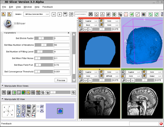 Screenshot of the MRIBiasFieldCorrection module in Slicer3 during development. The screenshot illustrates the application of the MRI Bias Field Correction on the SPL Atlas. Note that the interface was simplified for the production version. The top left window shows the mask used to defined the ROI where the correction will be applied. The top right window shows the rendering of the 3D model created using the mask. The bottom left window shows one slice in the input image. Note the intensity inhomogeneity from the bottom left corner (dark) to the top right corner (bright). The bottom right window shows the output image after the application of the MRI Bias Field Correction module. The parameters used for the correction are shown on the left panel of the Slicer3 interface. |
Module Description
The module filters the image to remove the intensity inhomogeneity due to the MRI image acquisition.
Usage
- Load the input dataset (Main menu: Add Volume)
- Create a Mask Volume using the Editor (Modules > Editor) (the Threshold tool should give a good result)
- Select the MRIBiasFieldCorrection module (Modules > Filtering > MRIBiasFieldCorrection)
- In the left panel, select the Input Volume
- Select the Mask Volume
- In the Preview Volume menu , select 'Create New Volume'
- Do the same for the Output Volume menu
- Modify the parameter values if desired (default values gave good results during our experiments)
- Click on Apply.
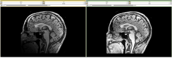 Close-up of the above screenshot showing the image before and after correction. Note that the intensity inhomogeneity visible in the input image (left) has been corrected in the output image (right). |
It took 32 min to process a 512x512x30 MRI volume on a MacBook laptop.
To visualize the result:
- Deselect the Overlay volume,
- Select the input as Background volume and the output as Foreground volume.
- Go to Modules > Volumes
- Select the input volume, and write down the values for Window and Level
- Select the output volume, and apply the same values
- Move the lower left cursor in 'Manipulate Slice Views' between B (background) and F (foreground)
Tests
On the Dashboard, these tests verify that the module is working on various platforms:
Known bugs
Links to known bugs in the Slicer3 bug tracker
Usability issues
Follow this link to the Slicer3 bug tracker. Please select the usability issue category when browsing or contributing.
Source code & documentation
Links to the module's source code:
Source code:
Doxygen documentation:
More Information
Acknowledgment
This work has been supported by NA-MIC (PI: Ron Kikinis).
References
- A Nonparametric Method for Automatic Correction of Intensity Nonuniformity in MRI Data, J.G. Sled, A.P. Zijdenbos, and A.C. Evans, IEEE Transactions on Medical Imaging, 17(1):87–97, Feb 1998.
- Parametric Estimate of Intensity Inhomogeneities Applied to MRI, M. Styner, C. Brechbhler, G. Szekely, and G. Gerig, IEEE Transactions on Medical Imaging, 19(3):153–165, Mar 2000.
- N4ITK: Nick's N3 ITK Implementation For MRI Bias Field Correction, Tustison N., Gee J., Insight Journal, 2009.


