Difference between revisions of "Modules:FourDImage-Documentation-3.6"
(Created page with 'Return to Slicer 3.6 Documentation __NOTOC__ ===Module Name=== 4D Analysis Module {| |[[Image:FourDAnalysisModuleScreenShot-3.5.png|thumb|280px|Screenshot…') |
|||
| (One intermediate revision by the same user not shown) | |||
| Line 1: | Line 1: | ||
[[Documentation-3.6|Return to Slicer 3.6 Documentation]] | [[Documentation-3.6|Return to Slicer 3.6 Documentation]] | ||
| + | |||
| + | [[Announcements:Slicer3.6#Highlights|Gallery of New Features]] | ||
__NOTOC__ | __NOTOC__ | ||
===Module Name=== | ===Module Name=== | ||
| − | 4D | + | 4D Image Module |
{| | {| | ||
| − | |[[Image: | + | |[[Image:FourDImage_Screenshot1.png|thumb|280px|'''Figure 1.''' Screenshot of 4D Image Module]] |
| − | |||
|} | |} | ||
| Line 25: | Line 26: | ||
===Module Description=== | ===Module Description=== | ||
| − | The 4D | + | The 4D Image module is designed to handle a time-series of 3D volume images (4D image), e.g. fMRI, cardiac images, dynamic contrast-enhanced (DCE) images in 3D Slicer. You can do: |
| − | * | + | *Load and save a series of 3D volume images from a directory, which contains multiple volume images. |
| − | * | + | *Scroll a 4D image in time direction. |
| − | * | + | *Edit (add, delete and insert) 3D frames in a 4D image. |
| − | In | + | The core component of 4D Image module is '''Time Series Bundle Node''', which is defined in [http://svn.slicer.org/Slicer3/trunk/Modules/FourDImage/vtkMRMLTimeSeriesBundleNode.h vtkMRMLTimeSeriesBundleNode.h] and [http://svn.slicer.org/Slicer3/trunk/Modules/FourDImage/vtkMRMLTimeSeriesBundleNode.cxx vtkMRMLTimeSeriesBundleNode.cxx]. This special MRML node is designed to hold pointers to the scalar volume nodes in the time series. In addition to them, the node also holds pointers to two scalar volume nodes for visualization. These two visualization scalar nodes contain byte arrays that are displayed in the 2D and 3D viewers; the arrays are overwritten by the array of the latest current 3D image frame, when the user scrolls the time-series. This approach gives a flexibility to use the existing frame works of image processing for each scalar volume nodes in the time-series data, and visualization such as volume rendering. The two visualization scalar nodes holds images for foreground and background layers. |
== Usage == | == Usage == | ||
| − | |||
===Quick Tour of Features and Use=== | ===Quick Tour of Features and Use=== | ||
| − | + | * '''Active 4D Bundle panel:''' This panel allows choosing the active time series bundle node from MRML scene. All operations on the rest of the panels are applied to this bundle node. If you choose "Create New TimeSeriesBundle", the module creates a time series bundle node with no volumes. You can add any volume nodes in the scene from the '''Editor''' panel. | |
| − | * '''Active 4D Bundle:''' | + | * '''Load / Save panel:''' This panel is used to load and save 4D images. To load a 4D image, first specify the directory that contains the volumes from "Brows Input Directory" dialog box, and then press "Load Series" button. |
| − | + | * '''Control panel:''' This panel provides sliders to scroll the 4D images in the time dimension. The panel allows scrolling foreground and background images independently. The module can also automatically scroll the images with interval specified in the entry in the panel. | |
| − | * ''' | + | * '''Editor panel:''' The panel allows editing a 4D image. The users can move, insert and delete volume images within a 4D image. |
| − | |||
| − | * ''' | ||
| − | |||
| − | * ''' | ||
| − | === | + | ==Tutorials== |
| − | + | This tutorial section will demonstrate: | |
| + | *Basic operations (loading, viewing and editing) | ||
| + | *Importing 4D data from external software using [[Modules:OpenIGTLinkIF-Documentation-3.4| OpenIGTLink]] | ||
| + | <br> | ||
| − | ====Step 1: | + | ===Basic operations (loading, viewing and editing)=== |
| − | + | ====Step 1: Open the module==== | |
| − | + | Choose '''4D Imaging''' in the category of '''4D''' in the module menu. | |
| − | + | {| | |
| − | + | |[[Image:FourDImage_Module.png|thumb|600px|'''Figure 2.''' 4D Image Module starting screen]] | |
| + | |} | ||
| + | ====Step 2: Load image==== | ||
| + | Open '''Load / Save''' panel, and click '''Browse Input Directory''' button with a folder icon. Slicer will show a dialog box for you to choose a directory that contains volume images. After choosing a directory, press '''OK''' button on the dialog box and press '''Load Series''' button in the module panel. | ||
| + | 3D Slicer will pop up the progress window and start loading the images. The module can read any formats that are supported by 3D Slicer. If the specified directory contains single-series DICOM data (some scanners produce time-series data without changing series number for each volume), the module analyses the DICOM headers and split the series into volumes automatically. | ||
{| | {| | ||
| − | |[[Image: | + | |[[Image:FourDImage_InputDirectorySelection.png|thumb|600px|'''Figure 3.''' A dialog box for directory selection]] |
|} | |} | ||
{| | {| | ||
| − | |[[Image: | + | |[[Image:FourDImage_Loading.png|thumb|600px|'''Figure 4.''' 3D Slicer shows progress window while loading a series of images from the specified directory.]] |
|} | |} | ||
| − | ====Step 3: | + | ====Step 3: Scroll image==== |
| − | + | You can scroll the 4D image in '''Control''' panel in the module. The panel has two scroll sliders (Figure 5 (A)), which allow you to scroll the foreground and background images independently, even if you are viewing the same time-series in both layers. The module automatically can scroll the 4D image with specified interval, when one of the automatic scroll buttons (Figure 5 (B)) is pressed. While scrolling, the icon on the button changes to the 'pause' icon as shown in Figure 6. Press the same button again to stop the automatic scroll. | |
| − | + | {| | |
| − | + | |[[Image:FourDImage_TimeScroll.png|thumb|600px|'''Figure 5.''' Scrolling the 4D image in the time direction using '''Control''' panel]] | |
| − | + | |} | |
{| | {| | ||
| − | |[[Image: | + | |[[Image:FourDImage_PlayButton.png|thumb|280px|'''Figure 6.''' The button shows 'pause' icon while the automatic scrolling is active. ]] |
| − | |||
|} | |} | ||
| + | ====Step 4: Edit time-series==== | ||
| + | The '''Edit''' panel is used to move, insert and delete images in the time-series (Figure 7). | ||
{| | {| | ||
| − | |[[Image: | + | |[[Image:FourDImage_Edit.png|thumb|600px|'''Figure 7.''' '''Edit''' panel in 4D Image module.]] |
|} | |} | ||
| − | + | To move an image on the list, select the image (Figure 8), and then press '''Move up''' or '''Move down''' button bellow the list (Figure 9). | |
| − | |||
{| | {| | ||
| − | |[[Image: | + | |[[Image:FourDImage_EditSelection.png|thumb|280px|'''Figure 8.''' Selecting an image to move.]] |
| + | |[[Image:FourDImage_EditMoveUp.png|thumb|280px|'''Figure 9.''' Moving the image up by pressing '''Move up''' button.]] | ||
|} | |} | ||
| − | + | To insert an image in the MRML scene to the time series, choose the image node from the '''Add node''' pull-down menu (Figure 10, 11), and press '''Add''' button (Figure 12). | |
| − | To | ||
| − | |||
{| | {| | ||
| − | |[[Image: | + | |[[Image:FourDImage_EditInsertSelection.png|thumb|200px|'''Figure 10.''' The pull-down menu to choose an image to insert.]] |
| + | |[[Image:FourDImage_EditInsertSelection2.png|thumb|200px|'''Figure 11.''' Choosing the image from the menu.]] | ||
| + | |[[Image:FourDImage_EditInsert.png|thumb|200px|'''Figure 12.''' Inserting the image into the time-series by pressing '''Add''' button.]] | ||
|} | |} | ||
| + | |||
| + | To remove an image from the time series, select the image on the list (Figure 13) and click '''Remove''' button(Figure 14). | ||
{| | {| | ||
| − | |[[Image: | + | |[[Image:FourDImage_EditRemoveSeleciton.png|thumb|280px|'''Figure 13.''' Selecting an image to remove form the time-series.]] |
| + | |[[Image:FourDImage_EditRemove.png|thumb|280px|'''Figure 14.''' Removing the image from the time-series by pressing '''Remove''' button.]] | ||
|} | |} | ||
| − | ====Step | + | ===Importing 4D data from external software using OpenIGTLink=== |
| − | + | ====Step 1: Setup example data and simulator to send 4D data==== | |
| + | Before start, please download and compile [http://www.na-mic.org/Wiki/index.php/OpenIGTLink/Library OpenIGTLink Library]. | ||
| + | The library is also available in the Slicer3-lib/OpenIGTLink-build directory. | ||
| + | |||
| + | The following tutorial uses an example client program and data available in [http://svn.na-mic.org/NAMICSandBox/trunk/4DModules/Examples NA-MIC SnadBox subversion repository]. In Linux and Mac OS X, you can obtain the source code and data by using the following command: | ||
| + | |||
| + | $ svn co http://svn.na-mic.org/NAMICSandBox/trunk/4DModules/Examples Examples | ||
| + | |||
| + | I recommend to create a build directory next to the source directory. Use CMake to generate a Makefile. | ||
| + | |||
| + | $ mkdir Examples-build | ||
| + | $ cd Examples-build | ||
| + | $ cmake -DOpenIGTLink_DIR=<OpenIGTLink binary directory> ../Examples | ||
| + | |||
| + | If the example program is successfully complied, you can find '''4DClient''' in the build directory. | ||
| + | |||
| + | <br> | ||
| + | |||
| + | ====Step 2: Configure OpenIGTLink IF==== | ||
| + | After launching 3D Slicer, open '''OpenIGTLink IF''' module (Figure 15) and create a connector (Figure 16). | ||
{| | {| | ||
| − | |[[Image: | + | |[[Image:FourDImage_TransOpenIGTLinkIF.png|thumb|280px|'''Figure 15.''' '''OpenIGTLinkIF''' module in 3D Slicer.]] |
| + | |[[Image:FourDImage_TransAddConnector.png|thumb|280px|'''Figure 16.''' Adding a connector by pressing '''Add''' button in '''OpenIGTLinkIF''' module.]] | ||
|} | |} | ||
| + | |||
| + | Configure the connector it as a server(Figure 17). In this tutorial, we use port number 18944 (default). | ||
| + | Then click '''Active''' check box to activate (Figure 18). The status shows '''Wait''', once the connector becomes active. | ||
{| | {| | ||
| − | |[[Image: | + | |[[Image:FourDImage_TransSetServer.png|thumb|280px|'''Figure 17.''' Configuring the connector as a server by clicking '''Server''' check box.]] |
| + | |[[Image:FourDImage_TransActive.png|thumb|280px|'''Figure 18.''' Activating the connector by clicking '''Active''' check box. The status becomes '''Wait'''.]] | ||
|} | |} | ||
| − | == | + | ====Step 3: Run the client program to transfer the 4D data==== |
| − | === | ||
| − | |||
| − | + | Run the client program from a terminal. If 3D Slicer and the client program are running on the same machine, the arguments for the client program should be: | |
| − | |||
| − | + | $ ./4DClient localhost 18944 2 ../Examples/img/ | |
| − | |||
| − | + | The client program sends 5 consecutive volume images to 3D Slicer. While the client program is sending the images, | |
| − | + | the status field in '''OpenIGTLInkIF''' indicates '''Connected''' (Figure 19). | |
| − | + | After the client program stops, check the image nodes on '''Data''' module. | |
| − | + | If 3D Slicer successfully receives the volume images, it shows scalar volume nodes named '''Heart-00?''' in the scene (Figure 20). | |
| − | + | {| | |
| − | + | |[[Image:FourDImage_TransConnected.png|thumb|280px|'''Figure 19.''' The status field indicates that the client and the connector are connected.]] | |
| + | |[[Image:FourDImage_TransTransConfirmData.png|thumb|280px|'''Figure 20.''' The images transfered from the client are listed in '''Data''' module.]] | ||
| + | |} | ||
| − | + | ====Step 4: Create and edit time-series bundle==== | |
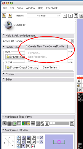
| − | + | Open '''4D Image''' module and create a new bundle node by choosing '''Create New TimeSeriesBundle''' from the '''Active 4D Bundle''' pull-down menu (Figure 21, 22). | |
| − | + | {| | |
| − | + | |[[Image:FourDImage_TransNewNode.png|thumb|280px|'''Figure 21.''' Choosing '''Create New TimeSeriesBundle''' to create a new bundle.]] | |
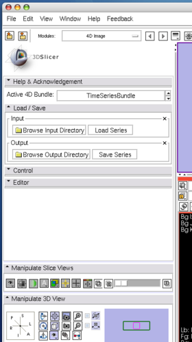
| − | + | |[[Image:FourDImage_TransNewNode2.png|thumb|280px|'''Figure 22.''' A new time series bundle is created.]] | |
| + | |} | ||
| − | + | Although you can manually add the images one by one as we did in the tutorial above, the module also allows specifying multiple nodes in the MRML by their name format. The format should be described in the same format used in printf() function in C. | |
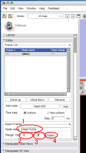
| + | In the '''Import Frames''' frame in '''Editor''' panel, put "heart128-%03d" in '''Node name''' field and set "0" and "4" in the '''Range fields''' (Figure 23). | ||
| + | Once '''Import''' button is pressed, the module adds the images into the time-series list (Figure 24). | ||
{| | {| | ||
| − | |[[Image: | + | |[[Image:FourDImage_TransImportFrames.png|thumb|280px|'''Figure 23.''' Specifying the format of node names and range of indexes.]] |
| + | |} | ||
| + | {| | ||
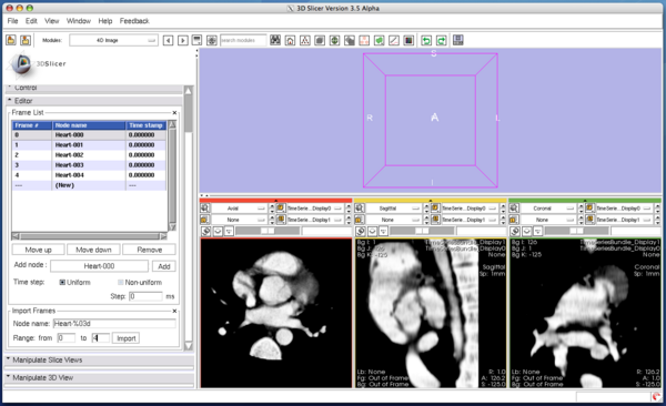
| + | |[[Image:FourDImage_TransImported.png|thumb|600px|'''Figure 24.''' The nodes are now listed in the time-series, after clicking '''Import''' button.]] | ||
|} | |} | ||
| − | + | <br> | |
| + | |||
| + | == Development == | ||
===Dependencies=== | ===Dependencies=== | ||
| − | + | This module does not require any other module. To import 4D image through network as demonstrated in the tutorial, you need to have [[Modules:OpenIGTLinkIF-Documentation-3.4| OpenIGTLink IF]] module. | |
===Known bugs=== | ===Known bugs=== | ||
| Line 153: | Line 190: | ||
== More Information == | == More Information == | ||
| − | |||
| − | |||
| − | |||
| − | |||
===Acknowledgment=== | ===Acknowledgment=== | ||
| − | This work is supported by NIH ( | + | This work is partly supported by NIH R21CA116271-02 (PI: Hiroto Hatabu), P01CA067165 (PI: Ferenc Jolesz), U41RR019703 (PI: Ferenc Jolesz), U54EB005149 (PI: Ron Kikinis) and P41RR013218-12 (PI: Ron Kikinis). |
===References=== | ===References=== | ||
Latest revision as of 21:58, 16 April 2010
Home < Modules:FourDImage-Documentation-3.6Return to Slicer 3.6 Documentation
Module Name
4D Image Module
General Information
Module Type & Category
Type: Interactive
Category: 4D
Authors, Collaborators & Contact
- Junichi Tokuda, Ph.D., Brigham and Women's Hospital
- Wendy J Plesniak, Ph.D., Brigham and Women's Hospital
- Ron Kikinis, M.D., Brigham and Women's Hospital
- Hiroto Hatabu, M.D., Ph.D., Brigham and Women's Hospital
Contact: Junichi Tokuda, tokuda at bwh.harvard.edu
Module Description
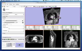
The 4D Image module is designed to handle a time-series of 3D volume images (4D image), e.g. fMRI, cardiac images, dynamic contrast-enhanced (DCE) images in 3D Slicer. You can do:
- Load and save a series of 3D volume images from a directory, which contains multiple volume images.
- Scroll a 4D image in time direction.
- Edit (add, delete and insert) 3D frames in a 4D image.
The core component of 4D Image module is Time Series Bundle Node, which is defined in vtkMRMLTimeSeriesBundleNode.h and vtkMRMLTimeSeriesBundleNode.cxx. This special MRML node is designed to hold pointers to the scalar volume nodes in the time series. In addition to them, the node also holds pointers to two scalar volume nodes for visualization. These two visualization scalar nodes contain byte arrays that are displayed in the 2D and 3D viewers; the arrays are overwritten by the array of the latest current 3D image frame, when the user scrolls the time-series. This approach gives a flexibility to use the existing frame works of image processing for each scalar volume nodes in the time-series data, and visualization such as volume rendering. The two visualization scalar nodes holds images for foreground and background layers.
Usage
Quick Tour of Features and Use
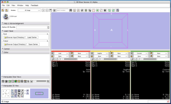
- Active 4D Bundle panel: This panel allows choosing the active time series bundle node from MRML scene. All operations on the rest of the panels are applied to this bundle node. If you choose "Create New TimeSeriesBundle", the module creates a time series bundle node with no volumes. You can add any volume nodes in the scene from the Editor panel.
- Load / Save panel: This panel is used to load and save 4D images. To load a 4D image, first specify the directory that contains the volumes from "Brows Input Directory" dialog box, and then press "Load Series" button.
- Control panel: This panel provides sliders to scroll the 4D images in the time dimension. The panel allows scrolling foreground and background images independently. The module can also automatically scroll the images with interval specified in the entry in the panel.
- Editor panel: The panel allows editing a 4D image. The users can move, insert and delete volume images within a 4D image.
Tutorials
This tutorial section will demonstrate:
- Basic operations (loading, viewing and editing)
- Importing 4D data from external software using OpenIGTLink
Basic operations (loading, viewing and editing)
Step 1: Open the module
Choose 4D Imaging in the category of 4D in the module menu.
Step 2: Load image
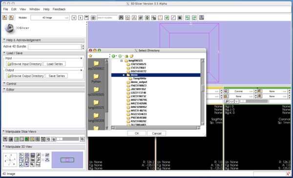
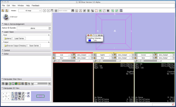
Open Load / Save panel, and click Browse Input Directory button with a folder icon. Slicer will show a dialog box for you to choose a directory that contains volume images. After choosing a directory, press OK button on the dialog box and press Load Series button in the module panel. 3D Slicer will pop up the progress window and start loading the images. The module can read any formats that are supported by 3D Slicer. If the specified directory contains single-series DICOM data (some scanners produce time-series data without changing series number for each volume), the module analyses the DICOM headers and split the series into volumes automatically.
Step 3: Scroll image
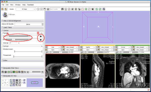
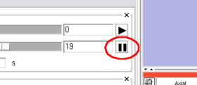
You can scroll the 4D image in Control panel in the module. The panel has two scroll sliders (Figure 5 (A)), which allow you to scroll the foreground and background images independently, even if you are viewing the same time-series in both layers. The module automatically can scroll the 4D image with specified interval, when one of the automatic scroll buttons (Figure 5 (B)) is pressed. While scrolling, the icon on the button changes to the 'pause' icon as shown in Figure 6. Press the same button again to stop the automatic scroll.
Step 4: Edit time-series
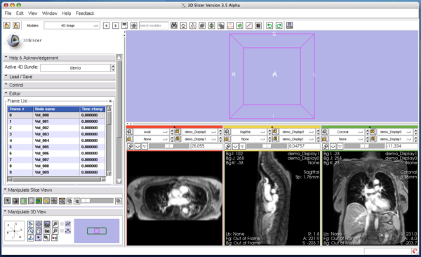
The Edit panel is used to move, insert and delete images in the time-series (Figure 7).
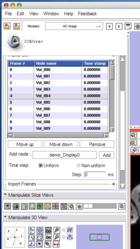
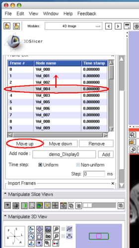
To move an image on the list, select the image (Figure 8), and then press Move up or Move down button bellow the list (Figure 9).
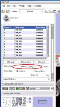
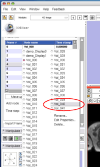
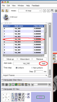
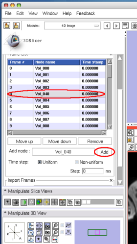
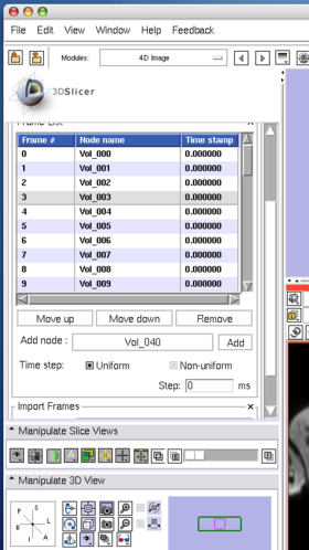
To insert an image in the MRML scene to the time series, choose the image node from the Add node pull-down menu (Figure 10, 11), and press Add button (Figure 12).
To remove an image from the time series, select the image on the list (Figure 13) and click Remove button(Figure 14).
Importing 4D data from external software using OpenIGTLink
Step 1: Setup example data and simulator to send 4D data
Before start, please download and compile OpenIGTLink Library. The library is also available in the Slicer3-lib/OpenIGTLink-build directory.
The following tutorial uses an example client program and data available in NA-MIC SnadBox subversion repository. In Linux and Mac OS X, you can obtain the source code and data by using the following command:
$ svn co http://svn.na-mic.org/NAMICSandBox/trunk/4DModules/Examples Examples
I recommend to create a build directory next to the source directory. Use CMake to generate a Makefile.
 $ mkdir Examples-build
 $ cd Examples-build
 $ cmake -DOpenIGTLink_DIR=<OpenIGTLink binary directory> ../Examples
If the example program is successfully complied, you can find 4DClient in the build directory.
Step 2: Configure OpenIGTLink IF
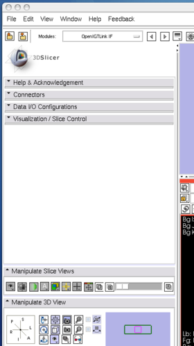
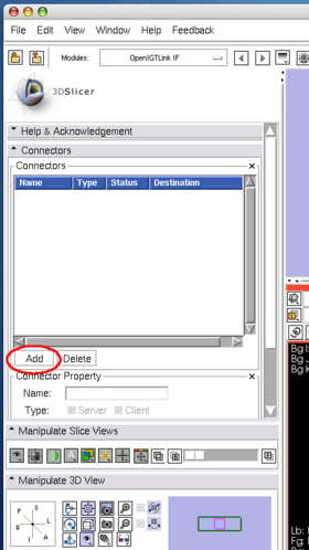
After launching 3D Slicer, open OpenIGTLink IF module (Figure 15) and create a connector (Figure 16).
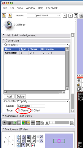
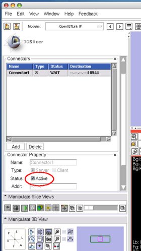
Configure the connector it as a server(Figure 17). In this tutorial, we use port number 18944 (default). Then click Active check box to activate (Figure 18). The status shows Wait, once the connector becomes active.
Step 3: Run the client program to transfer the 4D data
Run the client program from a terminal. If 3D Slicer and the client program are running on the same machine, the arguments for the client program should be:
$ ./4DClient localhost 18944 2 ../Examples/img/
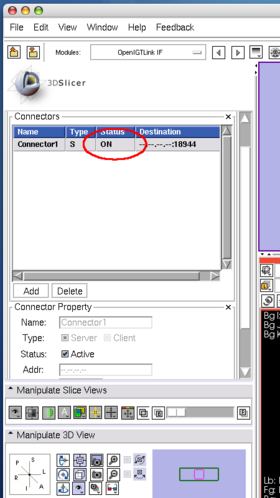
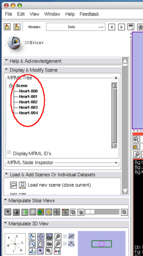
The client program sends 5 consecutive volume images to 3D Slicer. While the client program is sending the images, the status field in OpenIGTLInkIF indicates Connected (Figure 19). After the client program stops, check the image nodes on Data module. If 3D Slicer successfully receives the volume images, it shows scalar volume nodes named Heart-00? in the scene (Figure 20).
Step 4: Create and edit time-series bundle
Open 4D Image module and create a new bundle node by choosing Create New TimeSeriesBundle from the Active 4D Bundle pull-down menu (Figure 21, 22).
Although you can manually add the images one by one as we did in the tutorial above, the module also allows specifying multiple nodes in the MRML by their name format. The format should be described in the same format used in printf() function in C. In the Import Frames frame in Editor panel, put "heart128-%03d" in Node name field and set "0" and "4" in the Range fields (Figure 23). Once Import button is pressed, the module adds the images into the time-series list (Figure 24).
Development
Dependencies
This module does not require any other module. To import 4D image through network as demonstrated in the tutorial, you need to have OpenIGTLink IF module.
Known bugs
Follow this link to the Slicer3 bug tracker.
Usability issues
Follow this link to the Slicer3 bug tracker. Please select the usability issue category when browsing or contributing.
Source code & documentation
Customize following links for your module.
Links to documentation generated by doxygen.
More Information
Acknowledgment
This work is partly supported by NIH R21CA116271-02 (PI: Hiroto Hatabu), P01CA067165 (PI: Ferenc Jolesz), U41RR019703 (PI: Ferenc Jolesz), U54EB005149 (PI: Ron Kikinis) and P41RR013218-12 (PI: Ron Kikinis).
